xopr Demo Notebook - xopr Documentation

This is a basic demonstration of the core features of xopr for loading and plotting radar data.

%load_ext autoreload
%autoreload 2

import numpy as np
import xarray as xr
import geoviews as gv
import geoviews.feature as gf
import cartopy.crs as ccrs
import matplotlib.pyplot as plt

import xopr

import holoviews as hv
import hvplot.xarray
import hvplot.pandas
hvplot.extension('bokeh')

You’ll first establish an OPR session. This object serves to contain any needed information about how to connect to OPR and to the STAC API.

Generally, you can just use opr = xopr.OPRConnection(), but you may want to customize other options. The most common would be to create a local radar cache, which you can do as shown in the cell below.

If you specify a cache_dir, then fsspec will automatically manage a cache of any radar data that you need to download. This makes re-running things fast.

# Establish an OPR session
# You'll probably want to set a cache directory if you're running this locally to speed
# up subsequent requests. You can do other things like customize the STAC API endpoint,
# but you shouldn't need to do that for most use cases.
opr = xopr.OPRConnection(cache_dir="/tmp")

# Or you can open a connection without a cache directory (for example, if you're parallelizing
# this on a cloud cluster without persistent storage).
#opr = xopr.OPRConnection()

In the STAC catalog, every season (an entity such as 2022_Antarctica_BaslerMKB) is a distinct collection. You can list the available collections.

# List the available OPR datasets
collections = opr.get_collections()
print([c['id'] for c in collections])
selected_collection = '2022_Antarctica_BaslerMKB' # Select a collection for demonstration
print(f"Selected collection: {selected_collection}")

['2013_Greenland_P3', '2010_Antarctica_DC8', '2018_Greenland_P3', '2013_Antarctica_Basler', '2016_Greenland_G1XB', '2014_Antarctica_DC8', '2018_Antarctica_DC8', '2011_Greenland_P3', '2016_Antarctica_DC8', '2018_Antarctica_BaslerJKB', '2012_Greenland_P3', '2017_Antarctica_Basler', '2012_Antarctica_DC8', '2015_Greenland_C130', '2014_Greenland_P3', '2017_Greenland_P3', '2019_Antarctica_GV', '2016_Greenland_P3', '2019_Greenland_P3', '2011_Antarctica_DC8', '2024_Antarctica_GroundGHOST2', '2016_Greenland_Polar6', '2018_Antarctica_Ground', '2022_Antarctica_BaslerMKB', '2016_Greenland_TOdtu', '2011_Antarctica_TO', '2017_Antarctica_P3', '2013_Antarctica_P3', '2023_Antarctica_BaslerMKB']
Selected collection: 2022_Antarctica_BaslerMKB

Similarly, you can list available segments for a given season. We use the OPR terminology of segment to refer to a flight segment. In most cases, one segment corresponds to a single flight, but sometimes flights are broken into multiple segments for various reasons. A segment is uniquely defined by a collection (i.e. 2022_Antarctica_BaslerMKB) and a segment path (i.e. 20221212_01).

When we add a season into the STAC catalog, we add every segment for which a CSARP_standard product is available. (And we also link to other data products, if those are available.)

# List segments in the selected collection
segments = opr.get_segments(selected_collection)
print(f"Found {len(segments)} segments in collection {selected_collection}")
print(f"The first 3 segments are: {[s['segment_path'] for s in segments[:3]]}")

Found 23 segments in collection 2022_Antarctica_BaslerMKB
The first 3 segments are: ['20221210_01', '20221212_01', '20221213_01']

Once you pick a flight, we can actually start loading data. This happens in two steps. First, we get the STAC items, which are a description of the geometry and properties of each frame of data. They are returned from query_frames() as a GeoPandas GeoDataFrame.

selected_segment = '20230109_01' # Or from the list of segments like this: segments[0]['segment_path']
print(f"Selected segment: {selected_segment}")

stac_items = opr.query_frames(collections=[selected_collection], segment_paths=[selected_segment])
stac_items.head(3)

We can take a look at where our flight line is using the HoloViews accessor method to the GeoDataFrame.

background_map = gf.ocean.opts(projection=ccrs.SouthPolarStereo(), scale='50m') * gf.coastline.opts(projection=ccrs.SouthPolarStereo(), scale='50m')
background_map * stac_items.to_crs('EPSG:3031').hvplot(aspect='equal')

Now we’ll use the STAC items to actaully load radar data.

How much data this needs to transfer will vary depending on both how long the flight is and how the underlying data is stored. We’re working on migrating OPR data files to be cloud-optimized, however most of them aren’t and some of them are old-school MATLAB v5 files. xopr is designed to hide these differences from you as much as possible, but that can only go so far.

frames = opr.load_frames(stac_items)

Let’s look a single frame. This corresponds to a single .mat file that you might download from the OPR website. The structure of this should look familiar to you.

If you’ve tried directly loading one of these files in Python, you’ll probably know that there are some quirks. We try to handle those behind the scenes and give you a nicely-formatted xarray Dataset.

If you’ve never heard of xarray, this might be a good time to go read the xarray overview doc.

# Inspect an individual frame
frames[0].xopr

You can manually merge the Datasets if you like, but xopr.merge_frames() will do it for you. This helper function will return a list with one xr.Dataset per segment path or a single xr.Dataset if there is only one segment represented.

flight_line = xopr.merge_frames(frames)

## Combine the frames into a single xarray Dataset representing the flight line
#flight_line = xr.concat(frames, dim='slow_time', combine_attrs=merge_dicts_no_conflicts).sortby('slow_time')
flight_line.xopr

For visualizing radargrams, it’s helpful (i.e. we can make the plotting more efficient) if the slow time spacing is even. We can ensure this is true by doing some stacking along a fixed-time window:

stacked = flight_line.resample(slow_time='2s').mean()

This gives us uniform spacing in the slow_time dimension. This allows for more efficient plotting (imshow can only be used with fixed spacing -- try pcolormesh if your spacing is variable).

stacked = flight_line.resample(slow_time='2s').mean()

stacked['Data'] = 10*np.log10(np.abs(stacked['Data']))

stacked.xopr

OPR data often also includes traced layers (surface, bed, and occasionally internal layers). There are two distinct formats that OPR uses, which you may be familiar with from the CReSIS imb.picker tool. One is a database that stores layer picks. The other is a layer file that is available as a separate data product.

xopr allows you to fetch the relevant layer information from either source. To select only database layers, you can call get_layers(ds, source='db'). For layer files, you can call get_layers(ds, source='files'). By default, get_layers() will first look for a layer file and fall back to the database if a file cannot be found.

Once again, we do our best to hide the different formats. Once you’ve loaded the layers either way, you’ll get a dictionary mapping layer IDs to xarray Datasets of the same basic structure.

layers = opr.get_layers(stacked)

layers[1] # Display the surface layer as an example

We can also add vertical coordintes to the layers. By default, the layer information is provided in twtt (two-way travel time), but it can be helpful to transform this to range or WGS84 elevation.

Remember that layers is a dict where the keys are OPR layer identifiers. As such, 1 is always the surface and 2 is always the bed.

for layer_idx in layers:
    layers[layer_idx] = xopr.layer_twtt_to_range(layers[layer_idx], layers[1], vertical_coordinate='wgs84')
    layers[layer_idx] = xopr.layer_twtt_to_range(layers[layer_idx], layers[1], vertical_coordinate='range')

Finally, let’s make a radargram. If we were successful in loading layers, we will also plot the surface and bed layers here.

fig, ax = plt.subplots(figsize=(15, 4))
stacked['Data'].plot.imshow(x='slow_time', cmap='gray', ax=ax)
ax.invert_yaxis()

if layers:
    layers[1]['twtt'].plot(ax=ax, x='slow_time', linestyle=':', label='Surface')
    layers[2]['twtt'].plot(ax=ax, x='slow_time', linestyle='--', label='Bed')
    ax.legend()

ax.set_title(f"{stacked.attrs['collection']} - {stacked.attrs['segment_path']}")
plt.show()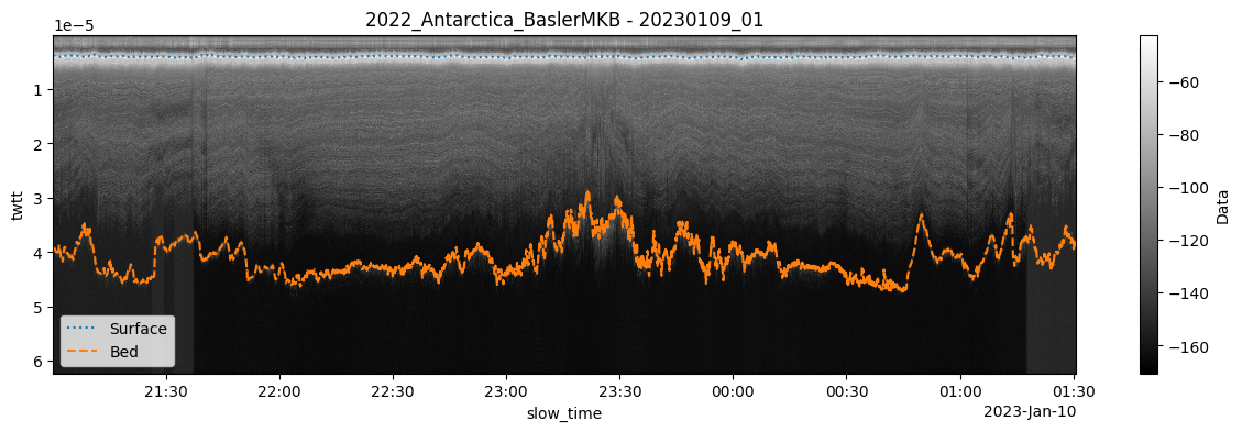

For display purposes, we can also transform the Y axis to show range (distance from the radar instrument, usually positive down) or altitude in WGS84 (negative down):

vcoord = 'wgs84' # Options are 'range' or 'wgs84'

tmp = xopr.interpolate_to_vertical_grid(stacked, vertical_coordinate=vcoord)

fig, ax = plt.subplots(figsize=(15, 4))
tmp['Data'].plot.imshow(x='slow_time', cmap='gray', ax=ax)
if vcoord == 'range':
    ax.invert_yaxis()

if layers:
    layers[1][vcoord].plot(ax=ax, x='slow_time', linestyle=':', label='Surface')
    layers[2][vcoord].plot(ax=ax, x='slow_time', linestyle='--', label='Bed')
    ax.legend()

ax.set_title(f"{stacked.attrs['collection']} - {stacked.attrs['segment_path']}")
plt.show()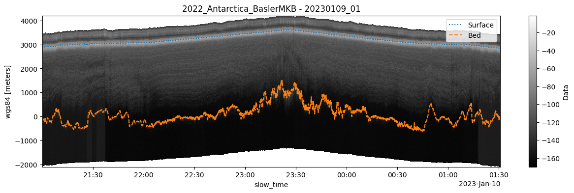

OPR data comes from many sources. Collecting and processing that data has required the contributions of many people over multiple decades. We want to make it easy for you, as a user, to figure out how to appropriately cite the data you’ve used. This is still just an early prototype, but here’s an idea of what it might look like to generate a report on how to cite your data:

print(flight_line.xopr.citation)

== Data Citation ==
This data was collected by The University of Texas at Austin.
Please cite the dataset DOI: https://doi.org/10.18738/T8/J38CO5
Please include the following funder acknowledgment:
This work was supported by the Center for Oldest Ice Exploration, an NSF Science and Technology Center (NSF 2019719) and the G. Unger Vetlesen Foundation.

== Processing Citation ==
Data was processed using the Open Polar Radar (OPR) Toolbox: https://doi.org/10.5281/zenodo.5683959
Please cite the OPR Toolbox as:
Open Polar Radar. (2024). opr (Version 3.0.1) [Computer software]. https://gitlab.com/openpolarradar/opr/. https://doi.org/10.5281/zenodo.5683959
And include the following acknowledgment:
We acknowledge the use of software from Open Polar Radar generated with support from the University of Kansas, NASA grants 80NSSC20K1242 and 80NSSC21K0753, and NSF grants OPP-2027615, OPP-2019719, OPP-1739003, IIS-1838230, RISE-2126503, RISE-2127606, and RISE-2126468.

xopr Documentation

Radar Data Availability

Notebooks

Searching by region and scaling up